Pytorch Learn

Hung-yi Lee

Pytorch.pdf & PyTorch中文文档

Tensor

Constructor

From list / numpy array

x = torch.tensor([[1,-1],[-1,1]])
x = torch.from_numpy(np.array([[1,-1],[-1,1]]))

Zero tensor

x = torch.zeros([2,2])    # [2,2] is shape

Unit tensor

x = torch.ones([1,2,5])  # [1,2,5] is shape

Operators

Squeeze: remove the specified dimension with length 1

>>> x = torch.zeros([1,2,3])
>>> x.shape
torch.Size([1,2,3])
>>> x = x.squeeze(0)  # dim = 0
>>> x.shape
torch.Size([2,3])

Unsqueeze:expand a new dimension

>>> x = torch.zeros([2,3])
>>> x.shape
torch.Size([2,3])
>>> x = x.unsqueeze(1) # dim = 1
>>> shape.shape
torch.Size([2,1,3])

Transpose:transpose two specified dimensions

>>> x = torch.zeros([2,3])
>>> x.shape
torch.Size([2,3])
>>> x = x.transpose(0,1)
>>> x.shape
torch.Size([3,2])

Cat:concatenate multiple tensors

>>> x = torch.zeros([2,1,3])    # dim_1 = 1
>>> y = torch.zeros([2,3,3])    # dim_1 = 3
>>> z = torch.zeros([2,2,3])    # dim_1 = 2
>>> w = torch.cat([x,y,z],dim=1)
>>> w.shape
torch.Size([2,6,3])             # dim_1 = 6

Addition 、Subtraction、Power、Summation、Mean

z = x + y
z = x - y
y = x.pow(2)
y = x.sum()
y = x.mean()

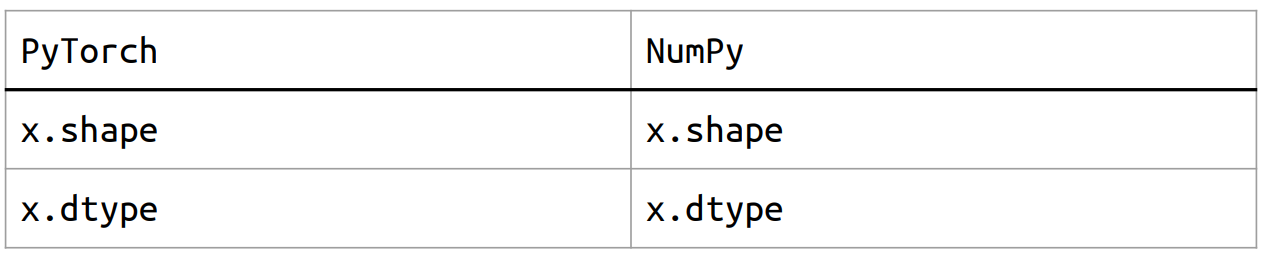
PyTorch v.s. Numpy

Attributes

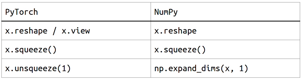
Shape manipulation

view 方法在改变张量形状时，要求新形状中的元素个数和原形状中的元素个数相同。此外，view 返回的是一个与原张量共享内存的视图。

import torch

# 创建一个 1D 张量
x = torch.arange(6)
print("Original tensor:", x)

# 使用 view 改变形状为 2x3
y = x.view(2, 3)
print("Reshaped using view:", y)

# 修改原张量的值，查看 view 对应的值
x[0] = 10
print("Modified original tensor:", x)
print("View after modifying original:", y)
# Original tensor: tensor([0, 1, 2, 3, 4, 5])
# Reshaped using view: tensor([[0, 1, 2],
#         [3, 4, 5]])
# Modified original tensor: tensor([10, 1, 2, 3, 4, 5])
# View after modifying original: tensor([[10, 1, 2],
#         [3, 4, 5]])

reshape 方法会返回一个新的张量，它可能会分配新的内存，而不是视图。它也允许一些灵活性，例如在某些情况下改变形状时，reshape 会自动进行内存的调整。

# 使用 reshape 改变形状为 2x3
z = x.reshape(2, 3)
print("Reshaped using reshape:", z)

# 修改原张量的值
x[1] = 20
print("Modified original tensor:", x)
print("Reshape after modifying original:", z)
# Reshaped using reshape: tensor([[10,  1,  2],
#         [ 3,  4,  5]])
# Modified original tensor: tensor([10, 20,  2,  3,  4,  5])
# Reshape after modifying original: tensor([[10,  1,  2],
#         [ 3,  4,  5]])

Device

Default: tensors & modules will be computed with CPU

CPU ：x = x.to('cpu')

GPU : x = x.to('cuda')

Check if your computer has NVIDIA GPU :torch.cuda.is_available()

Multiple GPUs: specify cuda:0, cuda:1, cuda:2, ...

How to Calculate Gradient?

Tensor自动求梯度+计算图模型+反向传播+Function对象

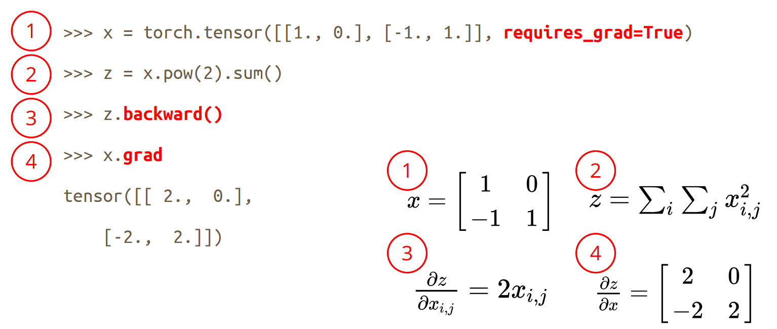
x = torch.tensor([1.0,0.],[-1.,1.],requires_grad=True)
z = x.pow(2).sum()
z.backward()
x.grad

在这段代码中，我们利用 PyTorch 进行自动求梯度，下面详细解释代码的每一个部分及其在反向传播中的作用。同时，我们也将介绍函数对象和叶子节点的概念。

1. 创建张量：

   x = torch.tensor([[1.0, 0.], [-1., 1.]], requires_grad=True)
   

   • 这里我们创建了一个二维张量 x，其内容是 [[1.0, 0.], [-1., 1.]]。
   • 设置 requires_grad=True，意味着我们希望跟踪这个张量的操作，以便进行自动求梯度。PyTorch 记录所有对该张量的操作，以便在反向传播时能够计算出梯度。
   • 此外， x 是一个叶子节点，这是指在计算图的最底层的张量，它是用户直接创建的张量或从其他张量分割而来，不是通过其他张量的操作结果产生的。

2. 定义计算图的输出：

   z = x.pow(2).sum()
   

   • x.pow(2) 是对 x 中的每个元素进行平方运算，生成一个新的张量，这个新张量并不是用户直接创建的，而是通过操作 x 生成，因此它不是叶子节点。
   • 接着，我们调用 .sum()，它会计算所有元素的和，结果保存在 z 中。至此，计算图已经构建完成，PyTorch 知道如何从 z 计算回 x。

3. 反向传播：

   z.backward()
   

1. 查看梯度：

   x.grad
   

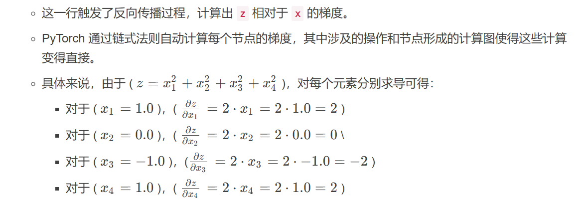
   • 这一行返回 x 的梯度，结果应为：tensor([[ 2., 0.], [-2., 2.]])。这对应于从反向传播过程中计算得到的梯度值。

• 在 PyTorch 中，任何通过运算生成的张量都可以看作是一个函数对象，它们代表了多个操作和计算结果的链表。例如，z 就是一个非叶子节点，它由 x 计算得到，而这些操作形成了一个计算图，这样在计算梯度时，我们就知道如何回溯。

Note 1：

从数据加载器（DataLoader）中得到的Tensor默认情况下其 requires_grad 属性是 False，这意味着这些Tensor在反向传播时不会计算梯度。这是因为输入数据通常不需要计算梯度，只有模型的参数（如权重和偏置）需要计算梯度以进行优化。

在计算损失的过程中，只有那些需要更新的模型参数（通常是权重，weight）的 requires_grad 属性设置为 True。这些参数在反向传播时会计算梯度，以便优化算法（如SGD、Adam等）可以使用这些梯度来更新模型参数。

整个过程可以简要总结如下：

1. 数据 Tensor 的 requires_grad 默认是 False，用于输入数据。
2. 模型参数（如权重）一般设置为 requires_grad=True，以计算梯度。
3. 损失函数的计算图仅涉及那些 requires_grad=True 的参数，进行反向传播时会计算梯度。

Note 2:

在 PyTorch 中，训练模型时传给损失函数（loss function）的参数通常是模型的输出（即预测值）和目标值（即真实标签）。从构建 Function 对象并用于反向传播的角度，我们可以更详细地理解这一过程。

首先，我们通过前向传播过程得到模型的输出，通常如下所示：

output = model(input_data)

output中是通过前向传播得来的，这个过程构建了计算图模型是一个Fucition对象，其中requires_grad=True的只有weight和bias这些parameter

在计算损失时，我们将模型输出和目标值传递给损失函数。例如，对于分类问题，常用的损失函数是 CrossEntropyLoss：

loss = loss_fn(output, target)

在 PyTorch 的底层，损失函数的计算是通过定义 Function 类来实现的。每个损失函数都会有一个与之关联的 Function 对象，它定义了前向传播（forward）和反向传播（backward）的方法。

• 前向传播：在前向传播时，损失函数将模型输出和目标值作为输入，计算损失值。这一过程记录了计算图的结构和数据流向。

• 反向传播：在反向传播时（当调用 loss.backward() 时），PyTorch 会使用在前向传播中记录的计算图来计算梯度。在这个过程中，框架会调用损失函数对应的 backward 方法，损失的梯度（对模型输出的梯度）会被传递回去，这个过程涉及计算链式法则，最终所有 requires_grad=True 的参数（如模型权重）都能得到相应的梯度。

在得到梯度后，我们使用优化器（如 SGD 或 Adam）来更新模型的参数。这一过程使用到计算过程中得到的梯度值。

optimizer.zero_grad()  # 清除之前的梯度
loss.backward()  # 反向传播，计算梯度
optimizer.step()  # 更新参数

Overview of the DNN Training Procedure

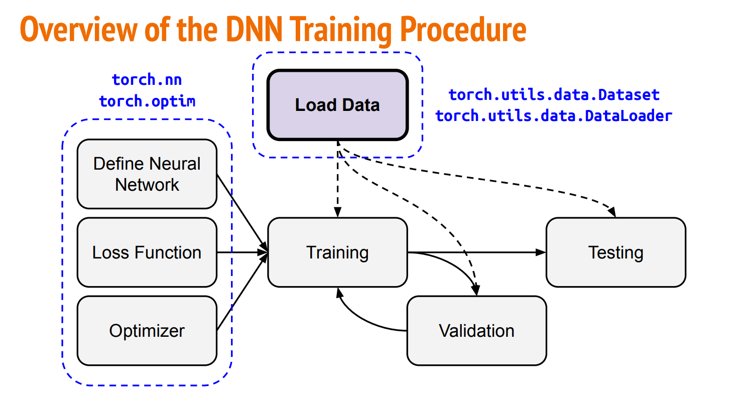
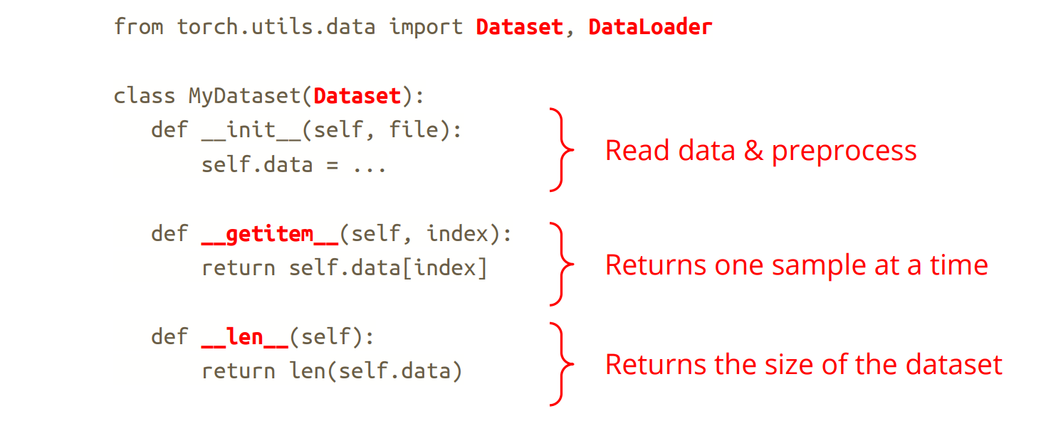
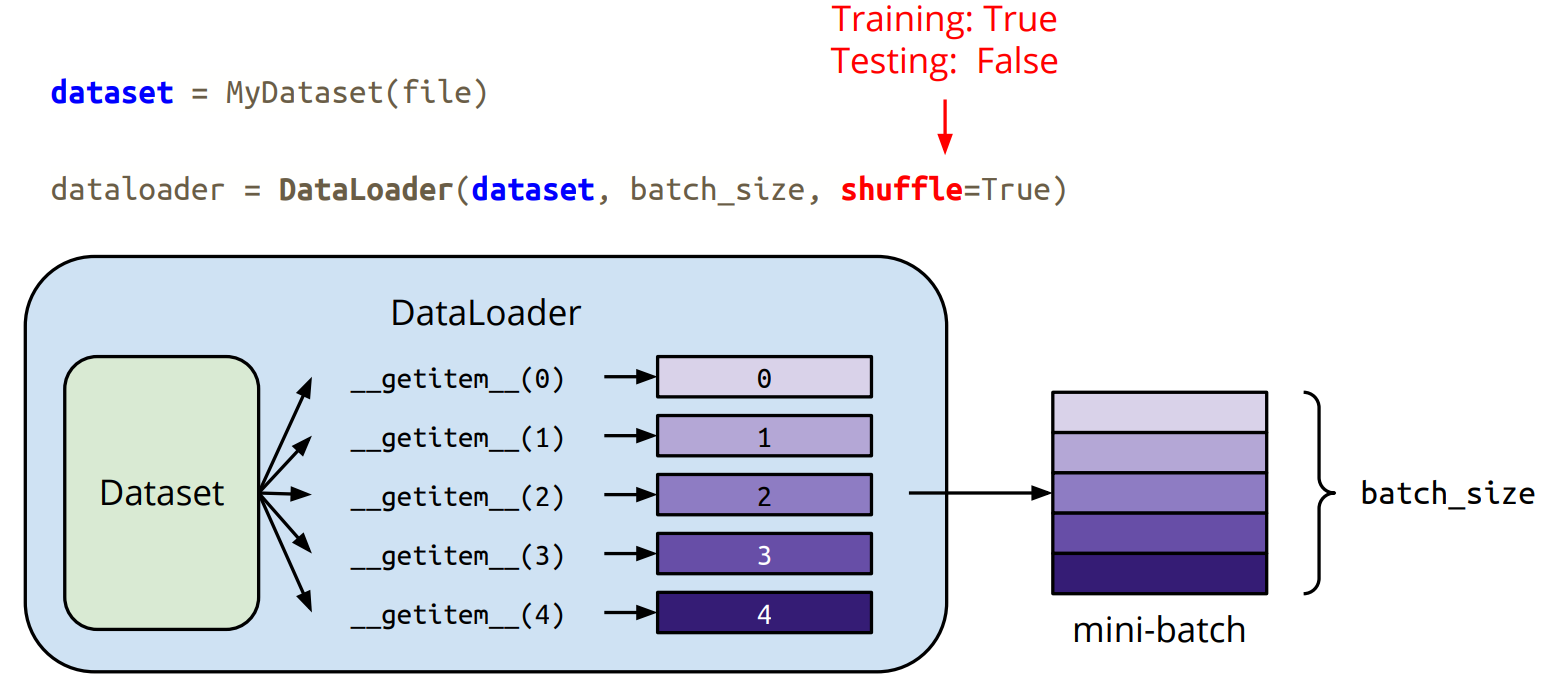
Dataset & Dataloader

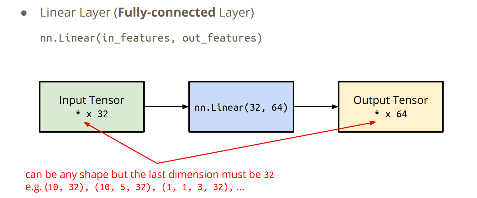
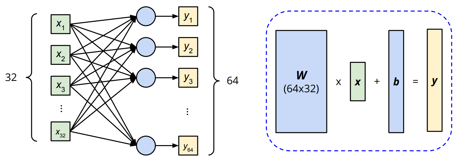
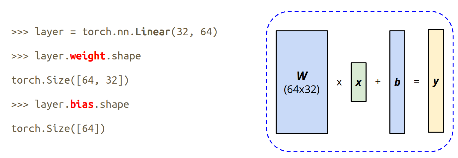
torch.nn

Neural Network Layers

nn.Module

Sequential接收一个 “子模块的有序字典（OrderedDict）”或者“一系列子模块”作为参数来逐一添加 Module 的实例，得到模型的forward 方法将这些实例按添加的顺序逐一计算，适用于模型的前向计算为简单串联各个层的计算的情况.

net = nn.Sequential(
        nn.Linear(784, 256),
        nn.ReLU(),
        nn.Linear(256, 10), 
        )

ModuleList 接收一个子模块的列表作为输入，可以类似 python List 那样进行 append 和 extend 操作

class MyModule(nn.Module):
    def __init__(self):
        super(MyModule, self).__init__()
        self.linears = nn.ModuleList([nn.Linear(10, 10) for i in range(10)])

    def forward(self, x):
        # ModuleList can act as an iterable, or be indexed using ints
        for i, l in enumerate(self.linears):
            x = self.linears[i // 2](x) + l(x)
        return x

ModuleDict 也是为了让网络定义 forward 时更加灵活而出现的，它接受一个子模块的字典作为输入，可以类似 python Dict 那样进行添加访问操作

net = nn.ModuleDict({
    'linear': nn.Linear(784, 256),
    'act': nn.ReLU(),
})

net['output'] = nn.Linear(256, 10) # 类似 python Dict 进行添加
print(net['linear'])               # 类型 python Dict 进行访问
print(net.output)                  # 另一种访问 key 'output' 的方法

print(net)
# net(torch.zeros(1, 784)) # 报NotImplementedError
# Linear(in_features=784, out_features=256, bias=True)
# Linear(in_features=256, out_features=10, bias=True)
# ModuleDict(
#   (linear): Linear(in_features=784, out_features=256, bias=True)
#   (act): ReLU()
#   (output): Linear(in_features=256, out_features=10, bias=True)
# )

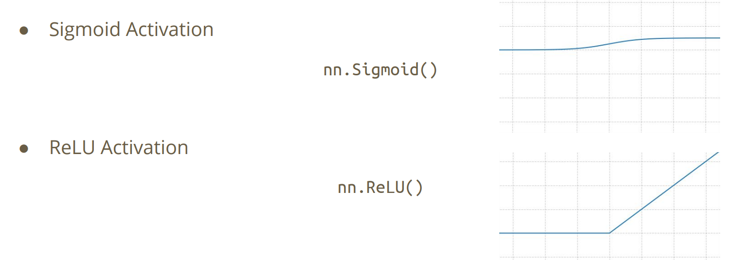
Activation Functions

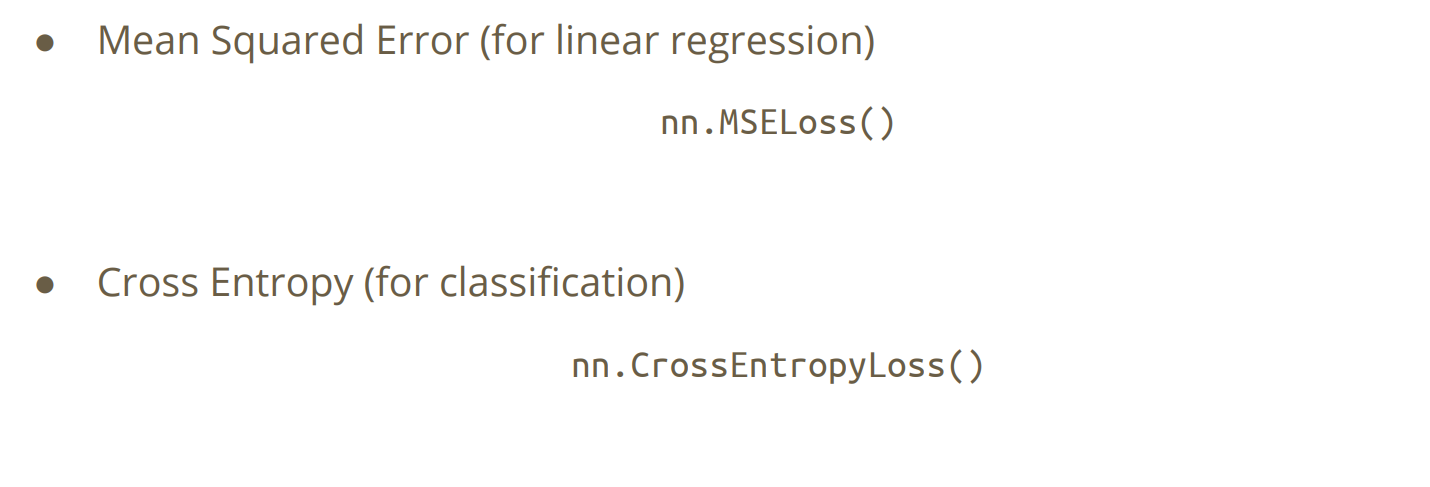
Loss Functions

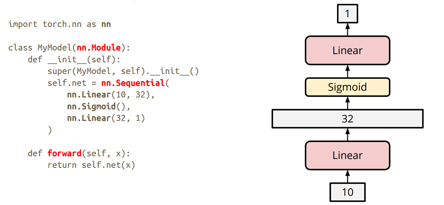
Build own neural network

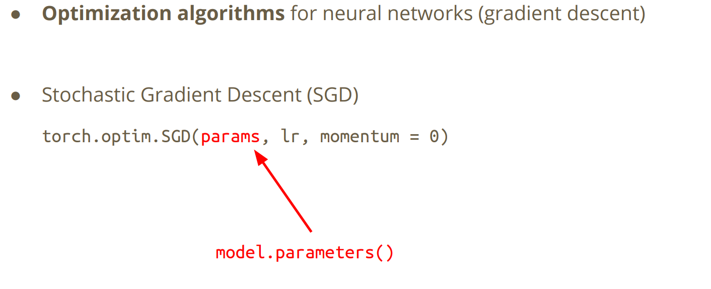
torch.optim

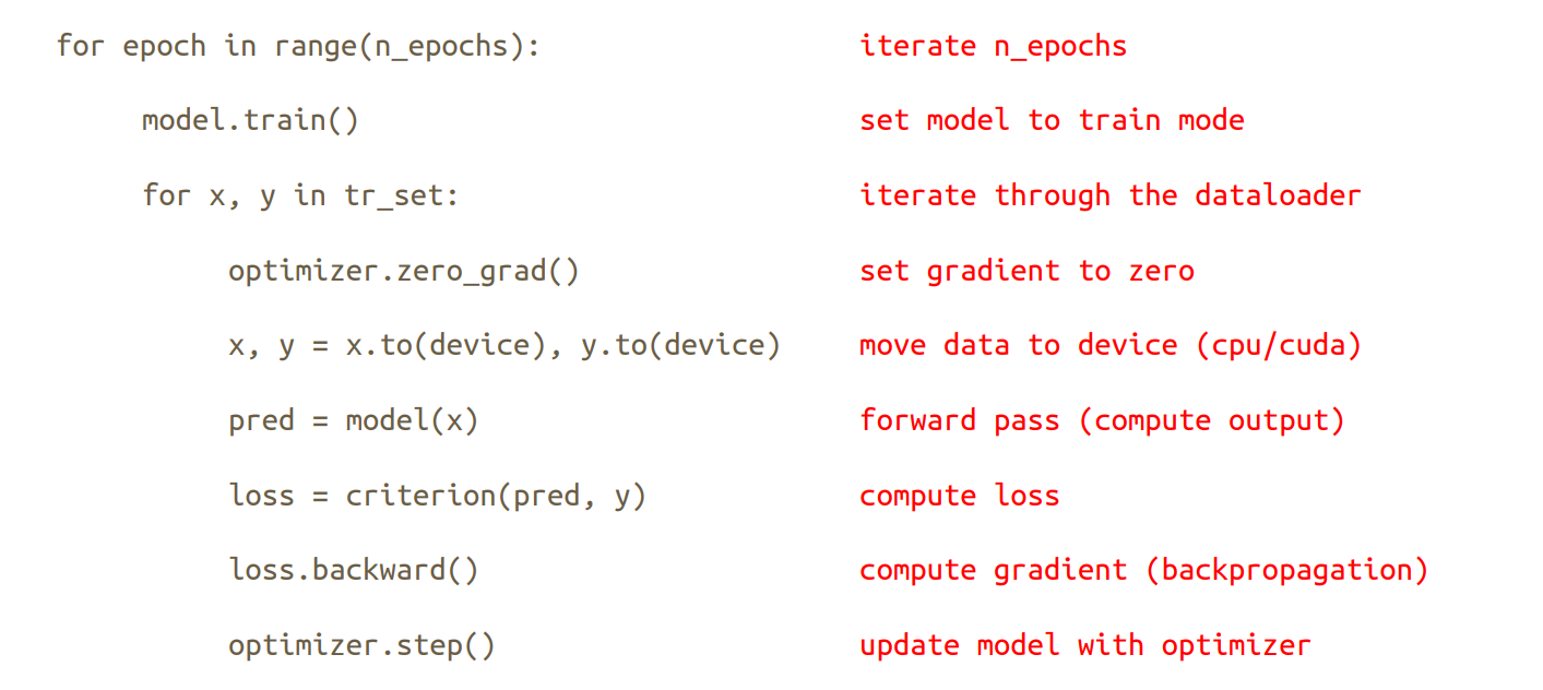
Neural Network Training

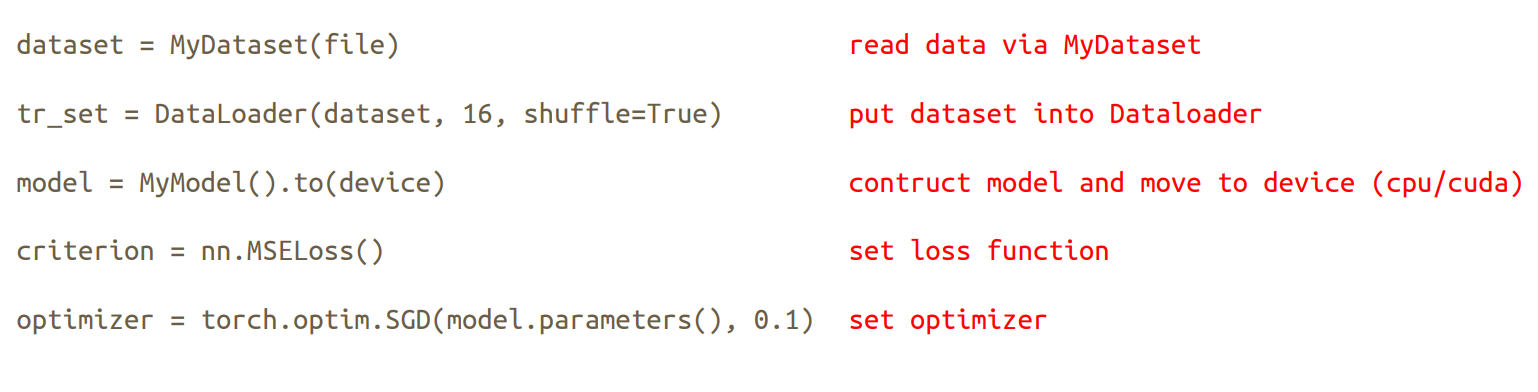
Neural Network Training

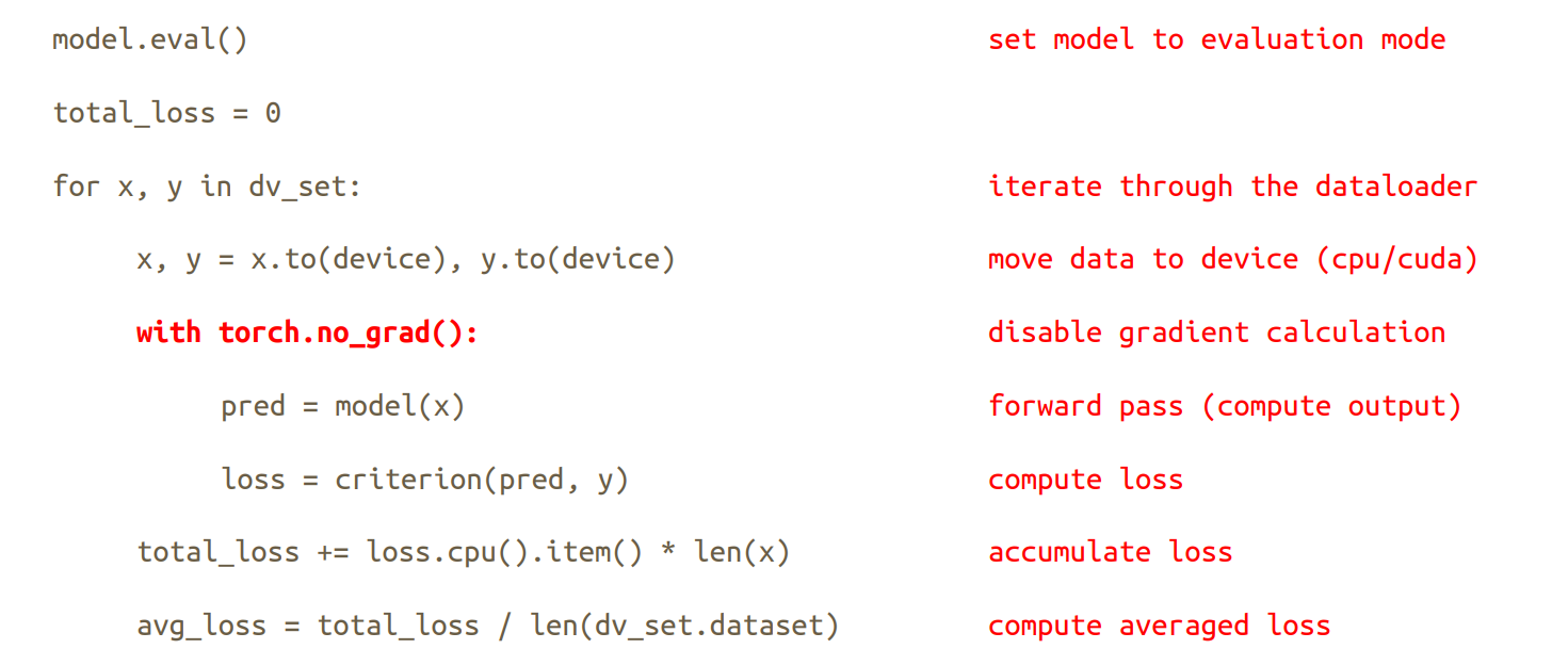
Neural Network Evaluation (Validation Set)

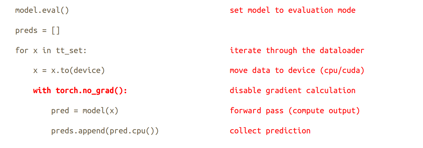
Neural Network Evaluation (Testing Set)

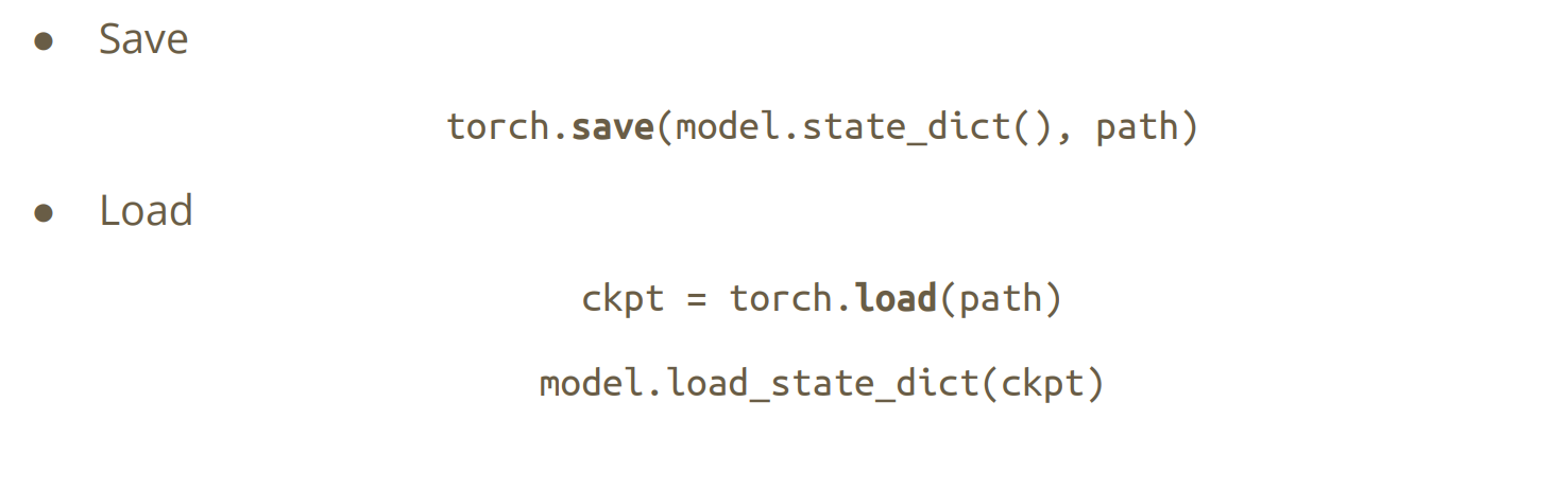
Save/Load a Neural Network